Introduction

Raytracing is one of the first theories of light propagation to ever
be developed. A ray, conceptually, represents the flow of power or
the path taken by “packet” of electromagnetic energy through a
system. Raytracing, more formally, is a reduction of Maxwell’s
equations to a much simpler and more computationally tractable form,
under fairly modest assumptions of smooth variation.

Raytracing has been used to study wave propagation and phenomena in
the ionosphere and magnetosphere for over 50 years
[Kimura(1966), Haselgrove(1955)].
Initially, the primary motivator was computational tractability. The
cost in computing a ray path in the magnetosphere is relatively small
compared to the cost of a global solution like that obtained using
finite difference or finite element methods. Initial investigations
were even carried out graphically
[Maeda and
Kimura(1956)].

In a modern context, however, raytracing is still a very important
computational tool for investigating magnetospheric phenomena. Due to
the enormous length scales (many megameters) and timescales (10s of
seconds), full simulations of wave propagation over the entire
magnetosphere are still difficult if not intractable on modern
computers.

Modeling efforts

The Stanford VLF group’s raytracing modeling efforts include:

Flexible raytracing simulation: The Stanford 3D ray tracer
can accommodate any arbitrary magnetic field or plasma density
function, opening up the possibility to study the role of
large-scale inhomogeneities, like plumes or notches, in the
propagation of VLF waves.

Modeling of loss and growth processes: Accurate modeling of
loss processes, like Landau and cyclotron damping, is essential to
accurate interpretation of raytracing results. The Stanford VLF ray
tracer can calculate the losses for any arbitrary distribution
function distributed over space, including observation-based models.

Physically-based and observation-based models: We have
integrated the IGRF, Tsyganenko, GCPM, and our own radial diffusion
model in our raytracer.

VLF Raytracing demonstrations

The VLF group at Stanford uses a 3D magnetospheric raytracer to study
many different wave propagation effects in the inner magnetosphere.
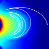
Ray paths in HF (as shown in Figure 1) show
characteristic total internal reflection off the ionosphere, an effect that is used for long-distance HF communication.

**Figure 1:**
Ray paths (white) taken by an HF source at 15 MHz, showing
reflection off the ionosphere. For reference, we also show the
log of the electron number density.

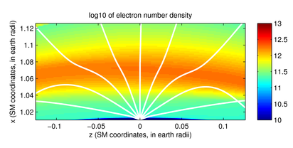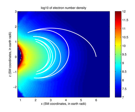
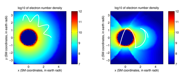
At VLF frequencies, however, the phenomena encountered are much richer
– rays can reflect off specular boundaries, magnetospherically
reflect, or even significantly drift in longitude, as shown in
Figures 2 and
3.

**Figure 2:**
Ray path (white) taken by a single VLF ray at 2 kHz using the GCPM
plasmasphere model and the IGRF+Tsyganenko-05 magnetic field
model, showing multiple magnetospheric reflections. The sun is at
the right (positive x direction).

**Figure 3:**
Left, poleward view of the path taken by a VLF ray at 150
Hz launched from sunside in the GCPM+IGRF+Tsyganenko-05 model,
showing significant longitudinal drift. Right, the same path from
a different view. In both views, the sun is to the right
(positive x direction).

A short movie here illustrates how VLF
waves can propagate and reflect in the magnetosphere, in real time:

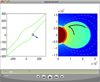
The panel on the left shows the refractive index surface, which is a
plot of the refractive index as a function of direction. The arrow in
blue on this plot shows the group velocity, or the direction of the
ray. On the right, we show the actual ray path superimposed on a
model-based electron density distribution with a very sharp
plasmasphere “knee”. The red arrow shows the direction of the
wavenormal, which in a plasma is not, in general, coincident with the
group velocity. A few interesting features can be seen clearly in
this visualization. Four of the reflections are termed MR
(magnetospheric reflections) and occur because the refractive index
surface’s topology changes from opened to closed, permitting an abrupt
change in the group velocity for a relatively small change in the
wavenormal at near-perpendicular propagation. The remaining two are
pseudo-specular reflections at the sharp plasmasphere boundary.

Bibliography

Haselgrove(1955)

Haselgrove, J. (1955), Ray Theory and a New Method for Ray Tracing, in
Physics of the Ionosphere, pp. 355-+.

Kimura(1966)

Kimura, I. (1966), Effects of Ions on Whistler-Mode Ray Tracing,
Radio Science, pp. 269-283.

Maeda and Kimura(1956)

Maeda, K., and I. Kimura (1956), A Theoretical Investigation on the
Propagation Path of the Whistling Atmospherics, Rept. Ionosphere
Res., pp. 105-123.