Introduction

Recent satellite-based measurements estimate that there are an average of $\sim$ 45 lightning flashes per second around the world (Christian et al., 2003).

Introduction

Recent satellite-based measurements estimate that there are an average of $\sim$ 45 lightning flashes per second around the world (Christian et al., 2003). The Stanford VLF group has recently developed a new methodology for a long-range lightning detection network capable of locating lightning flashes on a global scale with an accuracy usually associated with dense medium-range networks.

Lightning data finds many applications in both the scientific and commercial domains. Lightning flash rate has been coupled to mesocyclone evolution (Macgorman et al., 1989), storm size (Cherna and Stansbury, 1986), and convective rainfall rates (Tapia et al., 1998; Petersen and Rutledge, 1998). Lightning itself triggers many secondary processes in the upper atmosphere and magnetosphere whose study benefits from consistent high-resolution cloud-to-ground (CG) lightning data, including Lightning-induced Particle Precipitation (LEP) (Inan et al., 1985; Peter and Inan, 2007), sprites (Lyons, 1996; Inan et al., 1995), and terrestrial gamma-ray flashes (Cohen et al., 2010; Inan et al., 2006; Fishman et al., 1994). With sufficient location accuracy and low reporting latency, lightning detection networks may also be used as a tool to help mitigate the effects of lightning on electric power systems (Cummins et al., 1998a).

Lightning is an electrical discharge that partially neutralizes charge in a cloud. The current in a lightning channel also produces electromagnetic radiation at all frequencies from a few Hz (Burke and Jones, 1992) through to the optical band (Weidman and Krider, 1986). Various lightning detection networks measure specific portions of the electromagnetic spectrum, each with an associated set of benefits and trade-offs. Long-range lightning detection systems using sensors on the ground capable of detecting sferics $\sim$ 6000 km from the lightning discharge use the VLF portion of the electromagnetic spectrum, leveraging the particularly low attenuation through the Earth-ionosphere waveguide at these frequencies (Davies, 1990, p. 389).

Lightning Geo-Location

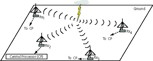
Figure 1 shows a cartoon of a lightning flash with four sensors, Rx1 through Rx4. In the general case, each receiver in the network estimates four parameters from each measured sferic: the arrival angle; the range between the receiver and the source location of the lightning discharge; the arrival time, measuring the GPS-referenced time of arrival of the sferic; and the amplitude (with polarity). These parameters are sent back to the central processor (CP), which then correlates them with measurements from other sensors to determine various parameters of the causative lightning discharge, such as the latitude and longitude on the earth’s surface, discharge time, and an estimate of peak current and polarity.

**Figure 1:**
Illustration of a cloud-to-ground lightning discharge generating a sferic which is sensed by four receiver stations, each with a communications link to a central processor.

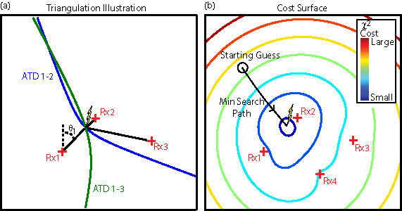
Using these four measurements, any number of stations can be used to estimate the discharge location and strength, though the estimates improve with greater redundancy. Figure 2a illustrates a simple approach using up to three receivers. First consider the case of a two-receiver network, using only Rx1 and Rx2. In this case the sferic arrival time difference (ATD), labeled as `ATD 1-2′ in the figure, between the two sensors defines a hyperbola (or a hyperboloid if the two sensors lie on an oblate spheroid, such as the earth), on which the lightning discharge position must occur. The location of the event along this curve is defined by the intersection of a projected azimuth line from one of the sensors, indicated by a black line in the figure. Adding a third station defines two ATD curves, which now intersect at two points defining two possible discharge locations. The ambiguity is generally best-resolved by adding the azimuth information. Adding a fourth station would define a third ATD line, which may not intersect with one of the two existing intersection points. The problem is over-determined, meaning that one can instead minimize a locally convex cost function over a constrained set of parameters. This type of minimization is illustrated in Figure 2b. A starting point is guessed, and, through an iterative procedure, the minimum point of the cost function is found and taken to be the lightning discharge’s location.

**Figure 2:**
Illustration of the triangulation procedure by (a) using intersecting arrival azimuth and/or arrival time difference curves and (b) finding the minimum of a cost surface.

Waveform Bank

The location accuracy in long-range lightning geo-location networks is heavily dependent on the arrival time accuracy. For an arrival time measurement uncertainty $\Delta t$ , the position of an ATD curve in Figure 2a moves
$\sim c\Delta t$ , where is the speed of light. For example, a 33 microsecond timing uncertainty gives a location uncertainty of $\sim$ 10 km. It is therefore important to reliably identify the arrival time of each sferic.

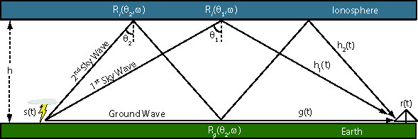
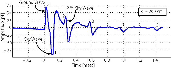
While the presence of the Earth-ionosphere waveguide enables detection of sferics at global distances, it also complicates our ability to consistently identify an arrival time. Sferic waveforms measured at each receiver may be represented by a convolution between a source term, determined by the current in the lightning channel itself, and a propagation term, governed by the specific path profile between the lightning discharge and the receiver. From a ray-hop perspective, the impulse response of the channel consists of a ground wave component and several ionospheric reflections (or “ray-hops”). Figure 3 illustrates the various components in this ray-hop model. The ground wave diffracts over the earth surface and has the shortest propagation distance. This wave is then followed by a succession of ray-hop sky waves.

**Figure 3:**
Illustration of the ground and multiple sky waves for a flat earth.

A sample measured waveform is plotted in Figure 4, showing the various components of the received waveform, including the ground wave and the successive sky waves. The ground wave, which has the most direct path, is seen arriving first, followed by the first sky wave, the second sky wave, and so on.

**Figure 4:**
Sample sferic that has propagated 700 km under a nighttime ionosphere. The ground wave and subsequent ionospheric reflections are labeled on the plot.

Using reference lightning discharge locations reported by the National Lightning Detection Network (NLDN) (Cummins et al., 1998b), we found that sferics from CG lightning discharges that propagate over the same path conform to a canonical shape. That is, for a fixed propagation path profile, the variability in the source waveform is sufficiently small such that an averaged sferic waveform is able to characterize a large percentage of the waveforms generated by negative CG strokes from a given storm cluster. This `canonical’ waveform shape varies as the path length changes and as the ionospheric profile changes from a daytime to nighttime profile (Said, 2009). The waveform structure has a weaker (though not negligible) dependence on the ground conductivity profile.

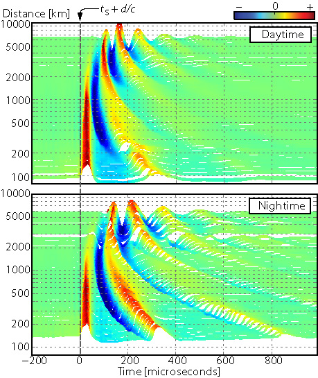
Figure 5 shows the empirically-derived canonical sferic waveforms for distances ranging from $\sim$ 100 km to $\sim$ 6,000 km, for both a daytime and nighttime ionosphere. Many of the features labeled in Figure 4 are easily identified in the waveform banks. The line labeled indicates the point in the time axis that corresponds to propagation at the speed of light. The ground wave emerges just after this line, then slowly attenuates into the noise at larger distances. As the distance increases, the difference in propagation path lengths between the ground wave and subsequent ionospheric hops decreases. As a result, these hops are seen to move in toward the ground wave with distance. At any given distance, the nighttime hops arrive later with respect to the corresponding daytime hops since VLF waves reflect at a higher altitude (and with a greater efficiency) under a nighttime ionosphere.

**Figure 5:**
Complete day and night waveform banks. Each row indicates a specific waveform bank entry. Each waveform has been normalized so that the maximum amplitude is unity. The time axis is referenced with 0 corresponding to a speed-of-light propagation; the distance index is plotted on a log scale to best capture the rate of feature changes.

This empirical “waveform bank” catalog is stored at each sensor and is used to accurately measure the arrival time of each sferic. When an incoming sferic is measured, it is compared to each entry in this waveform bank, analogous to a matched filter in a digital communication system (though the waveform bank entries are not orthogonal). When a good match is found, the receiver immediately has an estimate of the propagation distance and, more importantly, can identify each feature in the waveform. For short propagation distances, the sensor may report the rising edge of the ground wave. At larger distances, a component of one of the ionospheric hops is used. Since the specific feature is known, the central processor can adjust the arrival time estimate based on the approximate delay beyond the speed-of-light propagation time of the particular feature reported by the sensor.

The development of this technique utilized reference lightning discharge locations reported by NLDN to build up the empirical waveform bank and propagation delay corrections. While these results may be used for other propagation paths around the globe, a more accurate approach would be to use correction factors and/or waveform banks tailored to each possible propagation path at each sensor. There is ongoing research in the VLF group to build a more comprehensive database of possible sferic waveforms using both empirical measurements and numerical modeling. These results will help improve the location accuracy of a long-range network based on this methodology.

Trial Network and GLD360

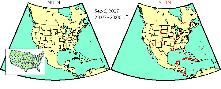
A three-sensor trial network, called the Stanford Lightning Detection Network (SLDN), was used to evaluate this approach to long-range lightning detection over the US. Figure 6 illustrates a qualitative check on the spatial coincidence between discharge locations identified by SLDN (on the right) and NLDN (on the left). One minute of data is plotted from each network. Most of the major storm clusters in NLDN are also identified by the SLDN. The NLDN data clusters over the landmasses, with a few additional discharges occurring in the ocean. SLDN additionally detects many events beyond the NLDN network coverage. The inset of the NLDN map shows a map of the NLDN sensor network; this map is to be compared to the three sensors used in the SLDN, indicated by green diamonds. The overall location accuracy over a 24-hour period for SLDN was found to be $\sim$ 2-4 km, with an NLDN-referenced detection efficiency between 40-60% (Said, 2009).

**Figure 6:**
Visual comparison between NLDN and SLDN strike locations for a one-minute period. Inset adapted from Cummins et al. (1998b).

Through a collaboration between Vaisala, Inc.
and the VLF group at Stanford, a new global lightning geo-location network based on this new methodology has recently been developed. This network, called GLD360, is professionally operated and maintained by Vaisala, Inc., which also operates the NLDN.

Acknowledgments

This work has been supported at various times by a Stanford Electrical Engineering Departmental Fellowship; grants from the National Science Foundation; a NASA Graduate Student Researchers Program Fellowship; and a collaboration agreement with Vaisala, Inc. Some of the data acquisition was supported by grants from the Office of Naval Research.

Bibliography

Burke, C. P., and D. L. Jones (1992), An experimental investigation of ELF attenuation rates in the earth-ionosphere duct, Journal of Atmospheric and Terrestrial Physics, 54, 243-250.
Cherna, E. V., and E. J. Stansbury (1986), Sferics rate in relation to thunderstorm dimensions, J. of Geophys. Res., 91, 8701-8708.
Christian, H. J., et al. (2003), Global frequency and distribution of lightning as observed from space by the optical transient detector, J. of Geophys. Res. (Atmospheres), 108(D1), 4-1, doi: rm10.1029/2002JD002347.
Cohen, M. B., U. S. Inan, R. K. Said, and T. Gjestland (2010), Geolocation of terrestrial gamma-ray flash source lightning, , 37, 2801-+, doi: rm10.1029/2009GL041753.
Cummins, K. L., E. P. Krider, and M. D. Malone (1998a), The US national lightning detection network $^{TM}$ and applications of cloud-to-ground lightning data by electric power utilities, IEEE Transactions on Electromagnetic Compatibility, 40(4), 465-480, doi: rm10.1109/15.736207.
Cummins, K. L., M. J. Murphy, E. A. Bardo, W. L. Hiscox, R. B. Pyle, and A. E. Pifer (1998b), A combined TOA/MDF technology upgrade of the U.S. national lightning detection network, J. of Geophys. Res., 103(D8), 9035-9044, doi: rm10.1029/98JD00153.
Davies, K. (1990), Ionospheric Radio, Peter Peregrinus Ltd.
Fishman, G. J., et al. (1994), Discovery of Intense Gamma-Ray Flashes of Atmospheric Origin, Science, 264, 1313-1316, doi: rm10.1126/science.264.5163.1313.
Inan, U. S., D. L. Carpenter, R. A. Helliwell, and J. P. Katsufrakis (1985), Subionospheric VLF/LF phase perturbations produced by lightning-whistler induced particle precipitation, J. of Geophys. Res., 90, 7457-7469.
Inan, U. S., T. F. Bell, V. P. Pasko, D. D. Sentman, E. M. Wescott, and W. A. Lyons (1995), VLF signatures of ionospheric disturbances associated with sprites, , 22, 3461-3464, doi: rm10.1029/95GL03507.
Inan, U. S., M. B. Cohen, R. K. Said, D. M. Smith, and L. I. Lopez (2006), Terrestrial gamma ray flashes and lightning discharges, , 33, 18,802-+, doi: rm10.1029/2006GL027085.
Lyons, W. A. (1996), Sprite observations above the U.S. High Plains in relation to their parent thunderstorm systems, , 101, 29,641-29,652, doi: rm10.1029/96JD01866.
Macgorman, D. R., D. W. Burgess, V. Mazur, W. D. Rust, W. L. Taylor, and B. C. Johnson (1989), Lightning rates relative to tornadic storm evolution on 22 may 1981., Journal of Atmospheric Sciences, 46, 221-251.
Peter, W. B., and U. S. Inan (2007), A quantitative comparison of lightning-induced electron precipitation and VLF signal perturbations, J. of Geophys. Res. (Space Physics), 112, 12,212-+, doi: rm10.1029/2006JA012165.
Petersen, W. A., and S. A. Rutledge (1998), On the relationship between cloud-to-ground lightning and convective rainfall, J. of Geophys. Res., 103(D12), 14,025-14,040, doi: rm10.1029/97JD02064.
Said, R. (2009), Accurate and efficient long-range lightning geo-location using a vlf radio atmospheric waveform bank, Ph.D. thesis, Stanford University.
Tapia, A., J. A. Smith, and M. Dixon (1998), Estimation of convective rainfall from lightning observations., Journal of Applied Meteorology, 37, 1497-1509.
Weidman, C. D., and E. P. Krider (1986), The amplitude spectra of lightning radiation fields in the interval from 1 to 20 MHz, Radio Sci., 21(6), 964-970.