Introduction

Modeling of VLF waves in the magnetosphere still remains a
computationally challenging task. Typical VLF waves may propagate for
many seconds in the magnetosphere over scales much larger than a
wavelength. In addition, nonlinear processes regularly give rise to
observable phenomena such as triggering, entrainment, and growth of
VLF waves. As such, computational modeling must be tailored to the
problem at hand. On medium scales, layered media models are most
appropriate.

Introduction

The first computational method applied to propagation of radio waves
in the earth’s magnetosphere was arguably raytracing. A few decades
ago, as computing power improved, so-called “moment methods” emerged
as the method of choice for solving complicated radiation or
scattering problems, but applying these methods to propagation in
general media like plasmas still remained a significant challenge.
Finite element methods (FEM) were also developed around this time and
began to be used for problems with complicated material shapes, but
development of explicit time-domain FEM for electromagnetics has
progressed slowly. In more recent decades, finite difference time
domain (FDTD) methods have become the method of choice, due to the
ease with which inhomogeneities or complicated materials (like
plasmas) can be handled. Interestingly, the FDTD method was first
applied to electromagnetics by K.S. Yee as early as 1966
[Yee(1966)], but
received little attention until RAM sizes became larger.

FDTD methods have been applied with great success to many complicated
problems in electromagnetics, including plasmas, photonics, antennas,
magnetospheric physics, etc. However, in recent years a more flexible
family of methods called “discontinuous Galerkin finite element
methods” (DG-FEM) have begun to gain acceptance in many areas that
were traditionally the stronghold of FDTD.

Discontinuous Galerkin Method

In the finite difference method, the operators (the derivatives) are
approximated:

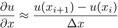$\displaystyle \frac{\partial u}{\partial x} \approx \frac{u(x_{i+1})-u(x_{i})}{\Delta x}$

The DG method, on the other hand, approximates the solution,
using a basis of expansion functions defined over a local finite element:

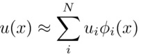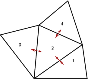
$\displaystyle u(x) \approx \sum_{i}^N u_i \phi_i(x)$

In the nodal DG framework
[Hesthaven and
Warburton(2008)], the solution is solved at
interpolation control points, as shown in the following figure:

**Figure 1:**
DG finite element showing interpolation control points.

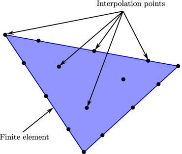
Each element is connected to its neighbors via a quantity called a
“flux,” which is related to some physical or abstract conserved
quantity in a system, e.g., conservation of mass in fluid mechanics,
or conservation of power in electromagnetics.

**Figure 2:** DG finite elements.
Element 2 is connected to its neighbors 1, 3, and 4 by exchanging flux
at the faces between the elements.

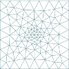
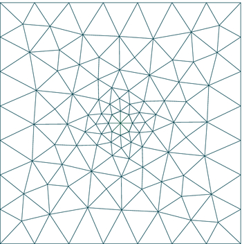
The entire domain is meshed to conform to the objects in the domain.
For instance, in the following figure, we show a mesh conforming to a
solid box with a small circle defined at the center:

**Figure 3:**
A domain meshed around a circle defined at the center of a
box.

The DG method has a number of interesting properties that make it
extremely well-suited for solving complicated equations:

Conformal meshes: Since the solutions are expanded
locally over each element, mesh elements can have any arbitrary
shape dependent on the problem geometry.

Colocated fields: In contrast to FDTD, high accuracy
does not require resorting to staggered grids.

Trivial parallelization: Parallelization only requires a
way to communicate the fluxes at the faces between elements on
different CPUs. That is, the stencil size is independent of the
order of accuracy.

Arbitrary order of accuracy: The order of accuracy can
be increased simply by increasing the number of basis functions in
the expansion.

DG in plasmas

The DG method can easily be used in plasmas. A so-called “cold
plasma” is characterized by a frequency-dependent plasma current:

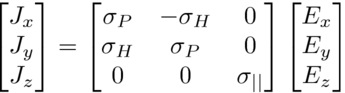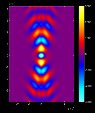
$\displaystyle \begin{bmatrix}J_x\\ J_y\\ J_z\end{bmatrix} = \begin{bmatrix} ... ...\sigma_{\vert\vert} \end{bmatrix} \begin{bmatrix}E_x\\ E_y\\ E_z\end{bmatrix}$

In the nodal DG framework, all that is required is to convert this
into a system of first-order ODEs, with plasma currents defined at
the interpolation control points. A sample 2D simulation showing an
antenna radiating into a magnetoplasma is shown below:

**Figure 4:**
A simulation of an antenna radiating into a cold
magnetoplasma. The magnetic field is oriented in the vertical
direction. The antenna is oriented perpendicular to the plane of
the plot.

DG-PIC

Real plasmas, of course, are not cold. Modeling all of the behavior
of real plasmas is still a major computational challenge, since the
entire velocity distribution of particles over the space must be taken
into account (a 6-dimensional space!), and many nonlinearities can
arise. Our current modeling efforts focus on using particle-in-cell
(PIC) techniques within the DG framework to incorporate these effects.
The PIC technique uses fields defined at fixed grid points to
move particles freely around. In turn, these particles form
a distribution of currents and charges, which are incorporated back
into Maxwell’s equations as extra source terms, as shown in the
following figure:

**Figure 5:** Illustration of the
classic PIC technique on a rectangular grid.

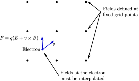
The primary advantage of using PIC within the DG framework is that the
approximate solution is defined everywhere, and is (in a
least-squares sense) the closest to the actual solution we can get
using a finite basis. We only need to reconstruct the solution using
the basis in order to find the fields at any point. In contrast, in
FDTD-PIC or finite volume-PIC, the fields must be interpolated, and
this only weakly connects a value to the actual approximate solution.

Bibliography

Hesthaven and Warburton(2008)

Hesthaven, J. S., and T. Warburton (2008), Nodal Discontinuous
Galerkin Methods.

Yee(1966)

Yee, K. (1966), Numerical solution of inital boundary value problems
involving maxwell’s equations in isotropic media, IEEE Transactions
on Antennas and Propagation, 14, 302-307,
doi:
rm10.1109/TAP.1966.1138693.